What is a Neural Network Explained: Beginner's Tutorial 2025

Ever wondered how artificial intelligence actually "thinks"? How does your phone instantly recognize your face, Netflix recommend the perfect movie, or a smart camera spot a delivery truck?

The answer, in most cases, is a neural network. These systems are the power behind the modern AI revolution, and they're modeled (loosely) on the human brain.

But what is a neural network?

At its core, a neural network is a powerful "pattern-finding" machine. It's a method in AI that teaches computers to process data in a way that is inspired by the human brain. These feedforward neural networks learn to recognize patterns, make decisions, and classify information through a process called training, all from being shown examples.

In this neural network basics for beginners 2025 guide, we'll demystify this technology completely. We won't get bogged down in heavy calculus. Instead, we'll use simple analogies and runnable code to build your intuition. We'll even see how these models are moving from giant data centers onto tiny devices, enabling a new wave of smart automation and AI-powered workflows.

You'll learn:

• How the biological inspiration of neural networks guides their design.
• What the core components—inputs, outputs, and hidden layers—actually do.
• How to build a neural network from scratch in PyTorch (it's easier than you think).
• The "magic" behind training a network to learn from its mistakes.
• How edge AI is using these concepts for real-time automation in 2025.

Prerequisites: All you need is some basic Python familiarity. No prior machine learning experience is required.

---

Table of Contents#

1. Biological Inspiration of Neural Networks
2. Neural Network Inputs and Outputs Explained
3. Hidden Layers—The Pattern Extraction Engine
4. Build Neural Network From Scratch PyTorch (XOR)
5. How to Train a Simple Neural Network
6. Edge AI Neural Networks for Automation
7. Quiz: Test Your Understanding

---

Step 1: Biological Inspiration of Neural Networks#

The term "neural network" isn't just a catchy name; it's a direct nod to its design. The entire concept is based on the biological inspiration of neural networks—specifically, the web of neurons in your brain.

The Theory: Brain vs. Model#

In your brain, you have billions of cells called neurons. Each neuron is connected to thousands of other neurons.

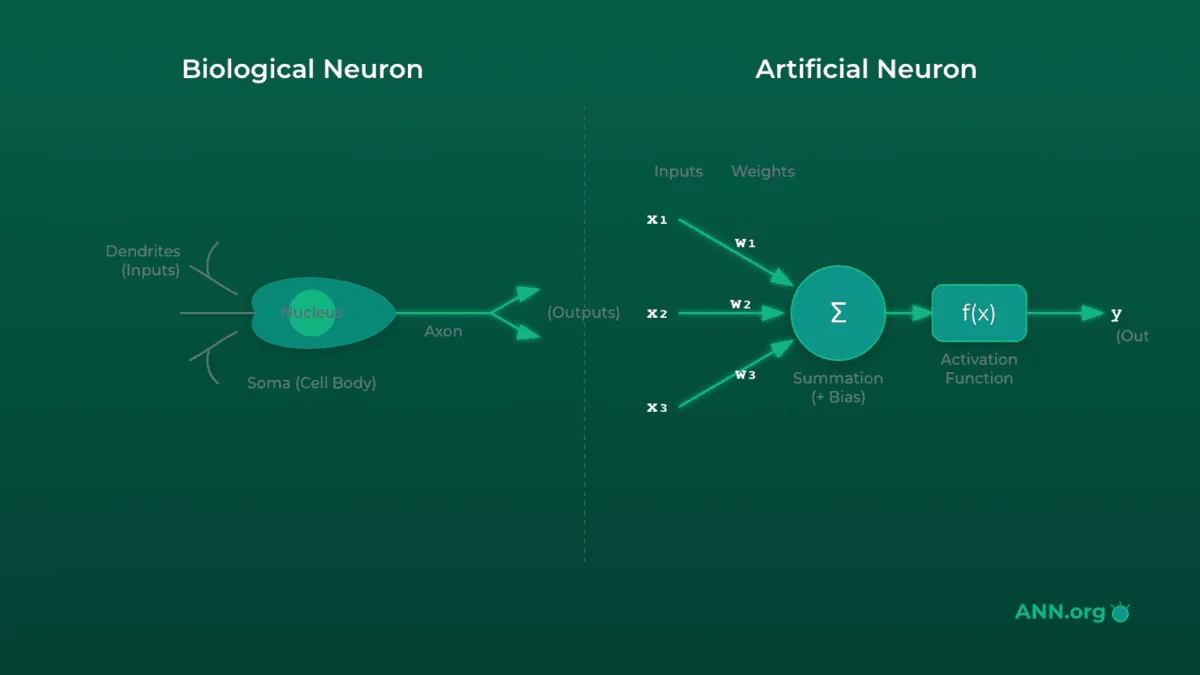
1. A neuron receives signals from other neurons through its dendrites (inputs).
2. It processes these signals in its cell body.
3. If the combined signal is strong enough (passes a threshold), the neuron "fires," sending its own signal out along its axon (output).
4. That signal crosses a gap, a synapse, to the next neuron, and the process repeats.

An artificial neuron (also called a perceptron in its simplest form) mimics this:

1. It receives one or more inputs (data).
2. Each input is multiplied by a weight, which signifies its importance. (This is like the "strength" of a synapse).
3. The node sums all the weighted inputs and adds a bias (a sort of thumb-on-the-scale to help it fire).
4. This sum is passed through an activation function (the "firing threshold") to produce the final output.

Analogy: The Dimmer Switch

Think of a single artificial neuron as a dimmer switch for a very smart light bulb.

• Inputs are people telling you to turn the light on.
• Weights are how much you trust each person. You trust your boss (weight = 0.9) more than a random stranger (weight = 0.1).
• The neuron sums these trusted "votes": (Boss's signal * 0.9) + (Stranger's signal * 0.1).
• The activation function is the switch itself. If the total "vote" score is above, say, 0.8, the light fires (turns on). Otherwise, it stays off.

Training a network is just the process of learning the right "trust" weights for all the switches.

The Code: A Single Neuron in Python#

Let's model this logic with a simple Python function. This isn't PyTorch yet—just the raw concept.

import math

def simple_neuron(inputs, weights, bias):
    """
    A simple neuron model:
    1. Calculates a weighted sum.
    2. Applies a Sigmoid activation function.
    """
    # 1. Calculate the weighted sum of inputs
    weighted_sum = 0
    for i, w in zip(inputs, weights):
        weighted_sum += i * w
    
    # 2. Add the bias
    weighted_sum += bias
    
    # 3. Apply the activation function (Sigmoid)
    # Sigmoid squashes any number into a value between 0 and 1
    output = 1 / (1 + math.exp(-weighted_sum))
    return output

# Example: A neuron deciding if a plant needs water
# Inputs: [sunlight (0-1), humidity (0-1), soil_moisture (0-1)]
# Weights: We "learned" these weights. Notice soil_moisture is negative.
#          It means HIGH moisture makes the neuron *less* likely to fire.
inputs = [0.8, 0.3, 0.1]
weights = [0.5, 0.2, -2.0] # Very sensitive to low moisture
bias = -0.5 # Neuron is slightly biased *against* firing

# Run the neuron
prediction = simple_neuron(inputs, weights, bias)

print(f"Neuron output: {prediction:.4f}")

# Interpret the result
if prediction > 0.5:
    print("Decision: Water the plant!")
else:
    print("Decision: Do not water the plant.")

# Try with dry soil
inputs_dry = [0.8, 0.3, 0.8] # Soil moisture is high
prediction_dry = simple_neuron(inputs_dry, weights, bias)
print(f"\n--- Dry Soil Test ---")
print(f"Neuron output: {prediction_dry:.4f}")
print("Decision: Do not water the plant.")

Real-world Tie: This simple "weighted decision" is the building block of everything. In a smart home, a neuron might decide to turn on the lights. Its inputs would be [motion_sensor, time_of_day, manual_override_switch]. The "weights" it learns determine how much it cares about motion versus the time of day.

---

Step 2: Neural Network Inputs and Outputs Explained#

A single neuron is just a switch. The real power comes from connecting thousands of them into a "network." This network is a data transformation pipeline. This section on neural network inputs and outputs explained will cover the start and end of that pipeline.

The Theory: The Data Pipeline#

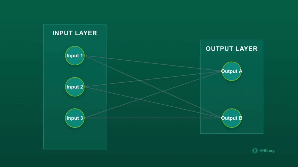
Every neural network has at least two layers:

1. Input Layer: This is the "front door" for your data. It doesn't make any decisions; it just formats your data into a numerical shape the network can understand.

   • Images: The inputs would be the pixel values (e.g., a 28x28 image becomes 784 input nodes).
   • Text: The inputs might be numerical IDs for each word.
   • Sensor Data: The inputs would be the sensor readings (like our plant example).

2. Output Layer: This is the "final result" layer. The number of nodes here depends entirely on your goal.

   • Regression (Predicting a number): One output node. (e.g., "predict house price").
   • Binary Classification (A or B): One output node (usually with a Sigmoid activation) representing the probability of class A. (e.g., "spam or not spam?").
   • Multi-class Classification (A, B, or C...): One output node for each class. (e.g., for recognizing digits 0-9, you'd have 10 output nodes). The one with the highest value is the network's prediction.

Analogy: The Digital Smoothie Maker

Think of the network as a fancy smoothie maker.

• Inputs are the raw ingredients you put in: strawberries, bananas, yogurt. You have to measure them in a format the machine understands: [grams_strawberries, grams_bananas, ml_yogurt]. This is your Input Layer.
• The machine (the network) blends and transforms them.
• Outputs are the final product. If your goal is regression (how many calories?), the output is one number: [350]. If your goal is classification (is this a fruit smoothie or a veggie smoothie?), the output is a probability for each: [prob_fruit: 0.9, prob_veggie: 0.1].

The Code: Defining Inputs/Outputs in PyTorch#

Let's use PyTorch, the most popular library for building NNs. We define our network's "shape" in a class.

nn.Linear(input_size, output_size) is PyTorch's way of creating a fully connected layer of neurons. It handles all the weights and biases for us.

import torch
import torch.nn as nn

# Define the network architecture as a class
class SimpleNetwork(nn.Module):
    def __init__(self, input_size, output_size):
        # Call the parent class's constructor
        super(SimpleNetwork, self).__init__()
        
        # Define our single layer of neurons
        # It takes `input_size` features and transforms them into `output_size` features
        self.layer = nn.Linear(input_size, output_size)

    def forward(self, x):
        # The forward() method defines how data flows *through* the network
        # Here, it just passes through our one layer
        return self.layer(x)

# --- Example 1: Regression Model ---
# Goal: Predict a single number (e.g., stock price) from 5 features
model_regression = SimpleNetwork(input_size=5, output_size=1)

# Create some dummy sensor data for one "sample"
# Note the [[...]] - PyTorch expects data in "batches"
sensor_data = torch.tensor([[0.2, 0.4, 0.1, 0.5, 0.9]]) 
print(f"--- Regression Model ---")
print(f"Input shape: {sensor_data.shape}")
output = model_regression(sensor_data)
print(f"Output: {output.item():.4f}")
print(f"Output shape: {output.shape}") # torch.Size([1, 1])

# --- Example 2: Classification Model ---
# Goal: Classify an item into 3 categories (e.g., "cat", "dog", "bird") from 10 features
model_classification = SimpleNetwork(input_size=10, output_size=3)

# Create dummy data
item_features = torch.tensor([[0.1, 0.2, 0.3, 0.4, 0.5, 0.6, 0.7, 0.8, 0.9, 1.0]])
print(f"\n--- Classification Model ---")
print(f"Input shape: {item_features.shape}")
output = model_classification(item_features)
print(f"Raw Outputs (Logits): {output}") # One number for each class
print(f"Output shape: {output.shape}") # torch.Size([1, 3])

# To get probabilities, we'd apply a function (e.g., Softmax)
probabilities = torch.softmax(output, dim=1)
print(f"Probabilities: {probabilities.detach().numpy()}")

Real-world Tie: In e-commerce, a model predicting if you'll buy an item might have inputs like [user_age, items_in_cart, time_on_page]. The output layer would be two nodes: [prob_will_buy, prob_will_abandon]. The network's entire job is to learn the connections between those inputs and the desired output.

---

Step 3: Hidden Layers—The Pattern Extraction Engine#

So, where does the "thinking" happen? If we just connect inputs to outputs, we have a very simple (and weak) model. The real power comes from hidden layers.

The Theory: Why We Need "Depth"#

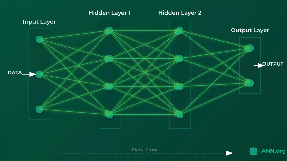
A hidden layer is any layer of neurons between the input and output layers. They are "hidden" because we don't directly feed them data or read their results; they are just part of the internal processing pipeline.

This is the "deep" in Deep Learning. More hidden layers = a deeper network.

Why use them? To learn complex patterns.

• A simple input-output model can only learn linear relationships (like "the more X, the more Y").
• Hidden layers allow the network to learn non-linear and hierarchical patterns.

In an image classifier, the layers learn progressively complex features:

• Hidden Layer 1 might learn to detect simple edges and curves.
• Hidden Layer 2 might learn to combine those edges into shapes (circles, squares).
• Hidden Layer 3 might learn to combine shapes into features (an "eye," a "wheel," a "nose").
• The Output Layer combines those features to make a final decision ("This is a face").

A crucial component here is the Activation Function (like nn.ReLU, Sigmoid, or Tanh). These activation functions introduce non-linearity—they're simple functions (e.g., "if input is negative, output 0, otherwise output the input") that are applied after each hidden layer. Without activation functions, the entire network would just collapse into one big, simple linear model, defeating the purpose of having layers.

Analogy: The Factory Assembly Line

Think of a network as a modern factory assembly line.

• Input Layer: The loading dock. It receives raw materials (e.g., pixels, sensor readings).
• Hidden Layer 1: The first station. It cuts the raw materials into basic shapes (e.g., "detects edges" or "finds a single keyword").
• Hidden Layer 2: The second station. It assembles those basic shapes into components (e.g., "combines edges into a circle" or "finds a phrase").
• Output Layer: The final station. It assembles the components into the final product and labels it (e.g., "This is a bicycle" or "This is a spam email").

Each layer specializes in one part of the task, building on the work of the previous one. This is what we'll build in this part of our neural network step by step tutorial.

The Code: A Deep Network in PyTorch#

Let's build a network for the famous MNIST dataset (handwritten digits). Each image is 28x28 pixels, and there are 10 possible outputs (digits 0-9).

• Input size: 784 (28 * 28)
• Output size: 10

import torch
import torch.nn as nn

class DeepNetwork(nn.Module):
    def __init__(self):
        super(DeepNetwork, self).__init__()
        
        # --- Define the Layers ---
        # 1. Input layer (784 features) to Hidden Layer 1 (128 neurons)
        self.hidden1 = nn.Linear(784, 128)
        
        # 2. Hidden Layer 1 (128 neurons) to Hidden Layer 2 (64 neurons)
        self.hidden2 = nn.Linear(128, 64)
        
        # 3. Hidden Layer 2 (64 neurons) to Output Layer (10 neurons)
        self.output = nn.Linear(64, 10)
        
        # Define the activation function we'll use
        # ReLU (Rectified Linear Unit) is fast and the most common choice.
        self.relu = nn.ReLU()

    def forward(self, x):
        # --- Define the Data Flow ---
        
        # 1. Pass data through Hidden Layer 1
        x = self.hidden1(x)
        # 2. Apply activation function
        x = self.relu(x)
        
        # 3. Pass data through Hidden Layer 2
        x = self.hidden2(x)
        # 4. Apply activation function
        x = self.relu(x)
        
        # 5. Pass to the Output Layer
        # No activation here; we'll apply it later (if needed)
        x = self.output(x)
        return x

# Create an instance of our network
model = DeepNetwork()
print(model)

# Create a dummy 28x28 image (flattened to 784)
# We use torch.randn to get random "pixel" data
dummy_image_data = torch.randn(1, 784) # 1 image, 784 pixels

# --- Test the flow ---
print(f"\nInput shape: {dummy_image_data.shape}")
output = model(dummy_image_data)
print(f"Output shape: {output.shape}")
print(f"Raw Output: {output}")

Real-world Tie: In productivity apps that filter spam, this is exactly how it works. The input is the text of an email. Hidden layers learn to spot patterns—not just a single word like "viagra" (which simple filters do), but combinations of features like ('urgent request' + 'unusual sender' + 'financial terms'). This requires the "deep" pattern-matching that hidden layers provide. To learn more about AI-powered automation, check out our AI blog.

---

Step 4: Build Neural Network From Scratch PyTorch (XOR)#

Let's put all the pieces together and build a neural network from scratch in PyTorch to solve a classic problem. This simple PyTorch neural network example will tackle the XOR logic gate.

The Theory: The XOR Problem#

XOR stands for "Exclusive OR." The logic is:

• 0 and 0 -> 0
• 0 and 1 -> 1
• 1 and 0 -> 1
• 1 and 1 -> 0

Why is this a big deal? Because it's non-linear. You can't draw a single straight line to separate the "0" results from the "1" results. This means our SimpleNetwork from Step 2 (with no hidden layers) cannot solve it. We must use a hidden layer.

Analogy: The VIP Doorman

The XOR problem is like telling a doorman to let in people who are wearing either a hat or a scarf, but not both.

• A simple rule (a linear model) fails. ("Let in anyone with a hat" wrongly includes 'hat and scarf').
• You need a two-step process (a hidden layer):
  1. Neuron 1 (Station 1a): "Is a hat present?"
  2. Neuron 2 (Station 1b): "Is a scarf present?"
  3. Output Neuron (Final Boss): "Are the answers from 1a and 1b different?"

This two-step logic is what our hidden layer will learn to do.

The Code: A Complete, Runnable XOR Network#

This is our first complete model. We'll define it here and then train it in the next step.

import torch
import torch.nn as nn

class XORNet(nn.Module):
    """
    A minimal neural network to solve the XOR problem.
    It has 2 inputs, one 4-neuron hidden layer, and 1 output.
    """
    def __init__(self):
        super(XORNet, self).__init__()
        
        # Input (2 nodes) -> Hidden (4 nodes)
        self.fc1 = nn.Linear(2, 4)
        
        # Hidden (4 nodes) -> Output (1 node)
        self.fc2 = nn.Linear(4, 1)
        
        # We'll use these activations in the forward pass
        self.relu = nn.ReLU()
        self.sigmoid = nn.Sigmoid() # Squashes output to 0-1

    def forward(self, x):
        # Pass through first layer and apply ReLU activation
        x = self.fc1(x)
        x = self.relu(x)
        
        # Pass through second layer and apply Sigmoid activation
        x = self.fc2(x)
        x = self.sigmoid(x)
        return x

# --- Test the network structure ---

# Initialize the model
xor_model = XORNet()
print("Model Architecture:")
print(xor_model)

# Define the 4 possible XOR inputs
# (A=0, B=0), (A=0, B=1), (A=1, B=0), (A=1, B=1)
# We need them as float tensors for PyTorch
test_inputs = torch.tensor([
    [0.0, 0.0],
    [0.0, 1.0],
    [1.0, 0.0],
    [1.0, 1.0]
])

# Test the *untrained* model
# The outputs will be random (around 0.5) because the weights
# haven't been "taught" the correct logic yet.
untrained_predictions = xor_model(test_inputs)

print("\n--- Untrained Predictions ---")
print(f"Inputs:\n{test_inputs.numpy()}")
print(f"Untrained Outputs:\n{untrained_predictions.detach().numpy()}")

Real-world Tie: While XOR is a textbook case, this exact structure is used constantly. Think of a smart thermostat deciding to turn on the AC. The inputs are [is_someone_home (0/1)] and [is_temp_above_75F (0/1)]. The desired logic might be to turn on the AC only if someone is home AND it's hot. This simple, non-linear decision is perfectly solved by a small network like this.

---

Step 5: How to Train a Simple Neural Network#

We've built a model, but its predictions are random. Now, we need to train it. This section explains how to train a simple neural network using the "training loop."

The Theory: Learning from Mistakes#

Training is a feedback loop where the network learns from its errors using a process called gradient descent.

1. Forward Pass: You give the network an input (e.g., [0, 1]) and it makes a guess (e.g., 0.52).
2. Calculate Loss: You compare the guess (0.52) to the true answer (1.0). The Loss Function (e.g., nn.BCELoss - Binary Cross-Entropy Loss) calculates an "error" score. A high score means a bad guess.
3. Backpropagation: This is the magic. The backpropagation algorithm calculates the gradient (think: "slope of the error") for every single weight inside it. This tells the network "to reduce the error, this specific weight needs to be increased a little, and this other one needs to be decreased a lot."
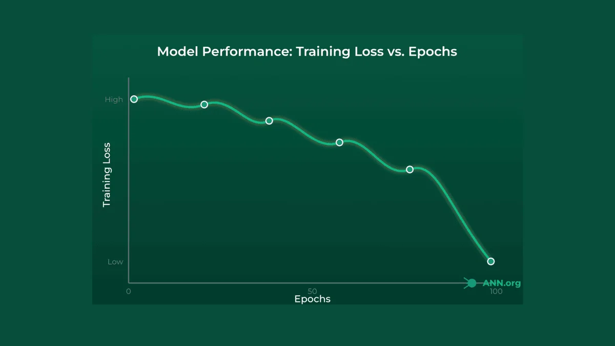
4. Optimizer Step: An Optimizer (e.g., optim.Adam using gradient descent) takes those gradients and "nudges" all the weights in the correct direction.
5. Repeat: You repeat this process thousands of times (called epochs). With each epoch, the network's guesses get slightly better, and the loss score goes down.

Analogy: Golfing in the Fog

Training a network is like playing golf in a thick fog.

1. Forward Pass: You can't see the hole, so you take a swing (make a prediction).
2. Calculate Loss: Your friend (the loss function) yells from the green, "You missed! Your ball is 50 feet to the left!" (This is your error score).
3. Backpropagation: You can't see the hole, but you can feel the slope of the ground under your feet (the gradient). You feel it slopes downhill to the right.
4. Optimizer Step: You adjust your stance and aim (update your weights) to hit slightly to the right, following the slope.
5. Repeat: You swing again (next epoch). Your friend yells, "Closer! Now you're only 10 feet away!" You repeat this loop until your loss is near zero.

The Code: A Full Training Loop#

Let's train the XORNet we just built.

import torch
import torch.nn as nn
import torch.optim as optim

# --- 1. Get our model and data ---
model = XORNet()

# Input data (X)
X = torch.tensor([
    [0.0, 0.0],
    [0.0, 1.0],
    [1.0, 0.0],
    [1.0, 1.0]
])
# Target labels (y)
y = torch.tensor([
    [0.0], # 0 XOR 0 = 0
    [1.0], # 0 XOR 1 = 1
    [1.0], # 1 XOR 0 = 1
    [0.0]  # 1 XOR 1 = 0
])

# --- 2. Define Loss Function and Optimizer ---
criterion = nn.BCELoss() # Binary Cross-Entropy Loss, good for 0/1 problems
optimizer = optim.Adam(model.parameters(), lr=0.01) # Adam is a popular, effective optimizer

# --- 3. The Training Loop ---
epochs = 5000 # How many times to "golf"

for epoch in range(epochs):
    # --- Step 1: Forward Pass ---
    # Make predictions on all 4 inputs at once
    predictions = model(X)
    
    # --- Step 2: Calculate Loss ---
    # How-to-train-a-simple-neural-network-model
    loss = criterion(predictions, y)
    
    # --- Step 3: Backpropagation ---
    # First, clear old gradients
    optimizer.zero_grad()
    # Now, calculate new gradients
    loss.backward()
    
    # --- Step 4: Optimizer Step ---
    # Nudge the weights
    optimizer.step()
    
    # Print progress
    if epoch % 500 == 0:
        print(f"Epoch {epoch}, Loss: {loss.item():.4f}")

# --- 4. Test the Trained Model ---
print(f"\nTraining finished! Loss: {loss.item():.4f}")
print("\n--- Trained Predictions ---")
# .detach() removes it from the "gradient-tracking" graph
trained_predictions = model(X).detach().numpy()

for i in range(len(X)):
    print(f"Input: {X[i].numpy()} -> Prediction: {trained_predictions[i][0]:.3f} (True: {y[i].item()})")

Real-world Tie: This exact loop is how massive image recognition models are trained. They are shown a picture of a cat (input), they guess 'dog' (prediction), the loss function says 'Wrong! Error = 0.9' (loss), backpropagation finds all the weights that contributed to 'dog', and the optimizer nudges them to be more 'cat'. Now, just repeat that 10 million times.

---

Step 6: Edge AI Neural Networks for Automation#

This brings us to one of the biggest trends for 2025: Edge AI. For years, AI models lived in "the cloud" on powerful servers. Now, we're running them on the device itself (your phone, your car, a factory sensor).

The Theory: AI On-Device#

"The Edge" refers to the edge of the network—the device in your hand, not a distant data center.

Why is this so important?

1. Speed (Latency): No internet lag. A self-driving car must identify a pedestrian instantly. It can't wait 500ms for a round-trip to the cloud to get a "Brake!" signal.
2. Privacy: The data (like your face, your voice) never leaves your device. It's processed locally.
3. Efficiency: It works even if your internet is down and saves on data costs.

This is the goal of edge AI neural networks for automation: to bring real-time, intelligent decision-making to the physical world, enabling instant, automated workflows.

Analogy: Cloud AI vs. Edge AI

• Cloud AI is like ordering from a restaurant. You send your order (data) to a big, powerful kitchen (the cloud). They cook it (process it) and send the meal (the result) back. It's powerful, but there's a delay, and you have to trust them with your order.
• Edge AI is like having a smart air fryer in your own kitchen. It's a small, highly-optimized appliance (a model on your edge device). You put food in, and it's cooked instantly. It's faster, private, and works even if your internet is out.

The Code: Exporting a Model for the Edge#

How do we "put the model on the device"? We train it (like in Step 5), and then we export it into a lightweight, optimized format. In PyTorch, this is often done with torch.jit.

import torch

# --- Assume 'model' is our fully trained XORNet from Step 5 ---
# (We'll just re-load it here for the example)
# model = XORNet() ... [training code] ...

# 1. Put the model in "evaluation" mode (disables training features)
model.eval()

# 2. "Script" the model using TorchScript
# This traces the model's 'forward' logic and saves it
# in a format that can run in other environments (like C++, mobile, etc.)
# We need a dummy input to show it the data shape
dummy_input = torch.tensor([[0.0, 0.0]])
scripted_model = torch.jit.script(model, dummy_input)

# 3. Save the model to a file
# This tiny file is what you would bundle into a mobile app
# or load onto a smart sensor (like a Raspberry Pi).
model_filename = "xor_model_for_edge.pt"
scripted_model.save(model_filename)

print(f"Model saved to {model_filename}")

# --- HOW AN EDGE DEVICE WOULD USE IT ---
print("\n--- Simulating Edge Device ---")

# The device (e.g., a C++ app) would only need this file.
# It doesn't need all the Python training code.
loaded_edge_model = torch.jit.load(model_filename)
loaded_edge_model.eval() # Set to evaluation mode

# An IoT sensor sends new, live data
sensor_reading = torch.tensor([[1.0, 0.0]]) # e.g., 'is_door_open', 'is_light_on'

# Run instant, local inference (no internet!)
with torch.no_grad(): # Disables gradient tracking for speed
    edge_prediction = loaded_edge_model(sensor_reading)

print(f"Edge device got input: {sensor_reading.numpy()}")
print(f"Edge device made prediction: {edge_prediction.item():.4f}")

Real-world Tie: This is the core of modern workflow automation. A quality-control camera on a factory line (edge device) runs a tiny exported model. It spots a defect in a bottle (local inference) and instantly triggers a robotic arm to remove it. It can't wait for a round-trip to the cloud. This is the future you're learning the foundation for right now.

---

Summary#

Congratulations! You've just gone from the biological concept of a neuron to building, training, and even exporting a neural network for a modern automation task.

Here are the key takeaways:

• Architecture: Neural networks are inspired by the brain. They pass data through an Input Layer, Hidden Layers (for pattern extraction), and an Output Layer (for the final decision).
• Training: The network "learns" by making guesses (forward pass), measuring its error (loss function), finding out how it was wrong (backpropagation), and nudging its weights to be better (optimizer).
• Implementation: Libraries like PyTorch make it easy to define complex network structures in just a few lines of Python.
• Applications (2025): The trend is moving "to the edge." By exporting models, we can run high-speed, private AI on small devices, enabling a new world of real-time automation.

The concepts you learned here—layers, activations, loss, and optimizers—are the fundamental building blocks for all deep learning, from ChatGPT to self-driving cars.